Symmetries and Order Parameters
Start out with a system (with properties and dynamics) described by its Hamiltonian \(\mathcal{H}\). \(\mathcal{H}\) is invariant under some group \(G\), which give the symmetries of \(\mathcal{H}\).
A system can have states with symmetries lower than the full group of the Hamiltonian, i.e. the state is invariant under some subgroup \(G\). We call those symmetry breaking.
Our state is described by thermodynamic (ensemble) averages of operators \(\phi_\alpha\), the ensemble average is then \(\langle\phi_\alpha\rangle,\langle\phi(x)\rangle\) which is not invariant under the full group \(G\).
These averages (⟨Φ⟩) are called order parameters. \(\langle\phi\rangle\) is a global order parameter and \(\langle\phi(x)\rangle\) is a local order parameter.
We can choose that the global order parameter is zero for high symmetry (always the full group, hence high T).
Symmetries
Discrete symmetries \(Z_2\), group 2 integers. Ex. Ising symmetries, uniaxial (anti-)ferromagnetic system. FM: \((\langle m_z\rangle)\). AFM: \(\langle m_{z,A}-m_{z,B}\rangle\). Ex: Rb \(_2\) NiF \(_4\), K \(_2\) MnF \(_4\). Order-disorder: Binary-order \(\langle n_A-n_B\rangle\) \([\beta-\text{brass}]\). Liquid-gas: \(\langle n_L-n_g\rangle\).
Dispacive: (Ferroelectric) perouskite \(\langle n_z\rangle\) BaLiO\(_3\).
\(Z_3\) group 3 integers. Graphene/ graphite surface (Krypton occupations on graphene lattice).
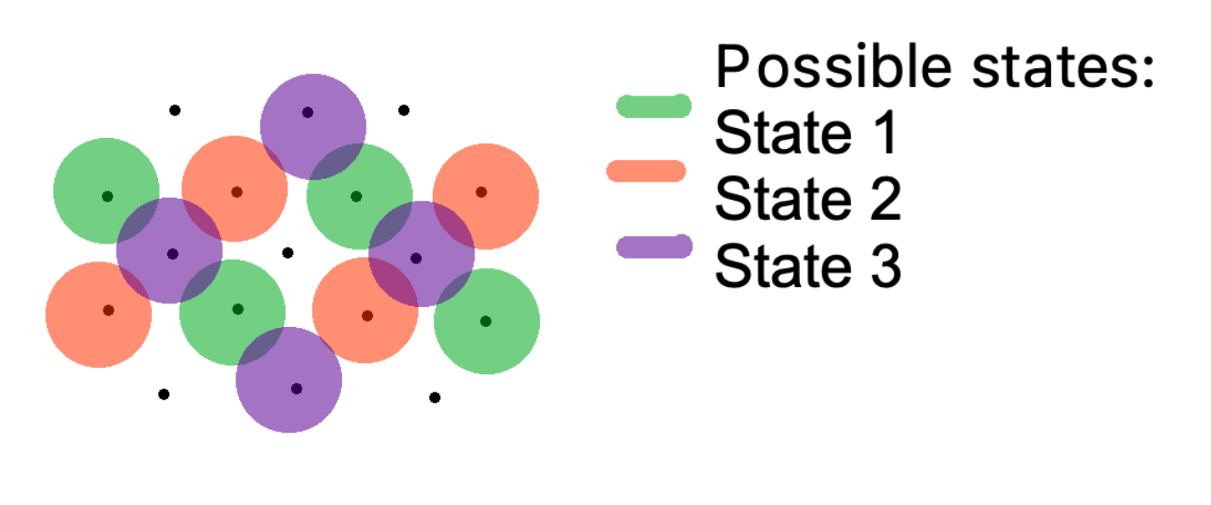
\(Z_N\) group \(N\) integers.
Continuous Symmetries:
- Rotations on a plane: O \(_2/U(1)\to\) Phase of a complex number.
Examples: Easy plane FM, Easy plane AFM, Bose-Einstein condensation (superfluid), various liquid crystal phases.
 \(O_3\) rotations in 3D, Heisenberg FM.
Axioms of Group
Set \(G\) with binary operatorion \(\cdot\). The group is \((G,\cdot)\).
- \(a(bc) = a(bc)\)
- \(a\cdot i = a\)
- \(a\cdot a^{-1} = i\)
Subgroup: Subset \(H\) to \(G\), \(H\) is a subscrube of \(G\) if \((H,\cdot)\) is also a group.
Towards Landau/ Landau-Gurburg Theory
\(F(\phi(x)) = \int d\overline{x} f(n(\overline{x}))\)
Consider if we have an ideal gas. Subdivide the space into boxes of size \(\Delta V\). Then for \(n_j\) points in the box at position \(\vec{x}_j\) we have the density, \(\rho(\vec{x}_j) = \frac{n_j}{\Delta V}\).
Consider a spatially inhomogenous system. (Ideal gas) with free energy \(F(T,V,N) = NkT\left(\ln\left(n\lambda^3\right)-1\right)\). \(N_j = n(\vec{x}_j)\Delta(V)\). \(f^{ig}=\frac{F(T,V,N)}{\Delta V} = n(\vec{x}_j)kT\left(\ln\left(n(\vec{x}_j)\lambda^3\right)-1\right)\) \(n(x), F[n] = \int f(n(x))dx\). We integrated out microscopic degrees of freedom and replaced with coarse-grained field. Can calculate any equilibrium property that can be written in terms of \(n(x)\). So, what is \(p(n(x)) = ?\). From before, \(\alpha\to p_\alpha(H)\). \(n(x)\to p(n(x))\) which is governed by the free energy \(F\) of the densities. \(p(n(x)) = \frac{1}{Z}\exp(-\beta F[n(x)])\). Driving force (to equilibrium)? \(\mu = \frac{\partial F}{\partial N} = \frac{\partial F/V}{\partial N/V} = \frac{\partial f}{\partial n}\). Then \(\mu(x) = \frac{\delta F[n(y)]}{\delta n(x)} = \frac{\delta}{\delta n(x)} \int f(n(y))dy\), which is called the variational/ functional derivative. Then, \(\mu(x) = kT\ln (n\lambda^3)\).
Considering currents. \(j = n\cdot v\), \(v \propto \frac{\partial\mu}{\partial x}\), \(v = -\gamma\frac{\partial\mu}{\partial x}\). \(\gamma\) relates to mobility and the negative relates to downhill. So, \(v = -\gamma n(x) \frac{\partial kT\ln(n(x)\lambda^3)}{\partial x} = -\gamma n(x)kT\frac{1}{n}\frac{\partial n}{\partial x}\). From the continuituy equation, \(\nabla\cdot J + \frac{\partial n}{\partial t} = 0\). Putting this together we get \(\frac{\partial n}{\partial t} = \gamma kT\frac{\partial^2 n}{\partial x^2}\).
\(F = \int dx f(T,\langle\phi(\overline{x})) + \int dx \frac{1}{2}k(\nabla\langle\phi(x)\rangle^2)\). Landau’s theory: ignore the second term. Including the second term is L-G.
So expanding, \(f(T,\phi) = f_0(T) + f_1\phi + f_2\phi^2 + f_3\phi^3 + f_4\phi^4 + \cdots\) where the coefficients \(f\) can depend on temperature, except:
- Highest power of \(\phi\) provides a bounding potential: \(\phi^{2n}, f_{2n}>0\). So that the order parameter remains finite.
- \(f_1\): example \(\phi = m = \frac{M}{V}\). \(F(T,V,M) \Rightarrow dF = -SdT - pdV + BdM\) \(\frac{\partial F}{\partial M} = \frac{\partial f}{\partial m} = B\). For high temperature and no field, the magnetization should be zero, hence \(\phi=0\). Then, \(\frac{\partial f}{\partial m}|_{m=0} = 0\) since it is a free energy minimum. Therefore, \(f_1 = 0\). Hence: \(f(T,\phi) = f_0(T) + f_2\phi^2 + f_3\phi^3 + f_4\phi^4 + \cdots\). \(f(T,\phi)\equiv\) Landau free energy density. This is typically written: \(f = f_0(T) + \frac{1}{2}\mu(T)\phi^2 + \frac{1}{3!}f_3\phi^3 + \frac{1}{4!}g\phi^4\) by theorists and partical physics. \(f = f_0(T) + \frac{1}{2}r\phi^2 - w\phi^3 + u\phi^4\). \(f = f_0(T) + \frac{1}{2}b(T)\phi^2 + \frac{1}{3}c(T)\phi^3 + \frac{1}{4}d\phi^4\).
Aside: MFT gives qualitative pictures that are pretty accurate to expectation.
Landau Model for Neumatic to Isotropic
Phase transition in liquid crystals.
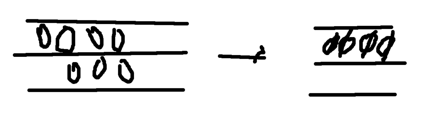
Isotropic: any orientation of liquid crytals. Neumatic: molecules predominantly align with some axis \(\hat{n}\).
Tensor Model - Neumatic to Isotropic Phase Transition in Liquid Crystal
Let \(\hat{n}\) be a global unit vector called the Frank director. Let \(\hat{v}^\alpha\) be the unit director for the \(\alpha\) molecule’s orientation.
Ordering is a measure of how close \(\hat{v}^\alpha\) is to \(\hat{n}\), \(\hat{v}^\alpha\cdot\hat{n} = \cos\theta\). For perfect order, \(\theta=0,\pi\) so \(\cos^k\theta\) with \(k\) even.
Want \(f = f_0 + f_1\phi + f_2\phi^2 + f_3\phi^3 + f_4\phi^4\).
In the high-temperature phase, \(f_1=0\).
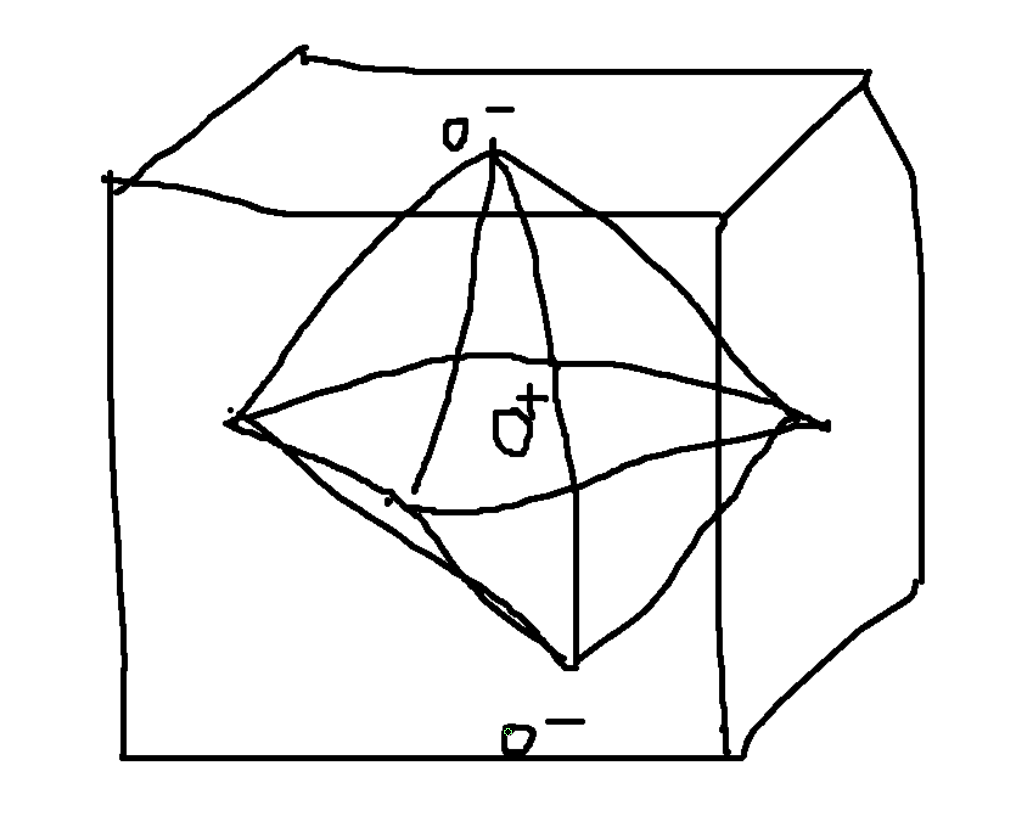
Let \(\mathcal{Q}\) be a tensor. Then, \(\phi^n = \text{Tr}\{\mathcal{Q}^n\}\). In high T phase \(\to \phi (high) = 0\). So, \(\text{Tr}\{\mathcal{Q}\} = 0\) for high temperature. So our outer product, \(\vec{v}\cdot\vec{v}^T\). Start with, \(\mathcal{Q}_{ij} = \sum_\alpha v_i^\alpha v_j^\alpha\). So, \(\mathcal{Q}(\vec{s}) = \frac{1}{\frac{N}{V}}\sum_\alpha v_i^\alpha v_j^\alpha\delta(x-\overline{x}^\alpha)\). Note the tensor must be symmetric.
Absolute disorder: \(\theta\) is uniformly distributed, \(\int d\Omega S(\theta) = 0\).
Absolute order, \(\forall\alpha.\vec{v}^\alpha\|\hat{n}\).
Choose a coordinate system such that the first basis vector is \(\hat{n}\). So perfect alignment is \(\vec{v}^\alpha = (1\: 0\: 0)\).
In order state, \(v^{\alpha T}v^\alpha\text{Tr}\left(\begin{pmatrix} 1 & 0 & 0 \\ 0 & 0 & 0 \\ 0 & 0 & 0 \end{pmatrix} + \begin{pmatrix} -1/3 & 0 & 0 \\ 0 & -1/3 & 0 \\ 0 & 0 & -1/3 \end{pmatrix}\right) = 0\).
\(\text{Tr}\left(\begin{pmatrix} S & 0 & 0 \\ 0 & 0 & 0 \\ 0 & 0 & 0 \end{pmatrix} + \begin{pmatrix} -S/3 & 0 & 0 \\ 0 & -S/3 & 0 \\ 0 & 0 & -S/3 \end{pmatrix}\right) = \text{Tr} \begin{pmatrix} 2/3S & 0 & 0 \\ 0 & -1/3S & 0 \\ 0 & 0 & -1/3S \end{pmatrix}\).
Then, \(\langle\mathcal{Q}_{ij}\rangle = S\left(n_in_j - \frac{1}{3}\delta_{ij}\right)\)
\(\int d\Omega S(\cos^k\theta) = 0 = \int d\varphi\int d\theta\sin\theta S(\cos^k\theta) = 2\pi\int d\theta\sin\theta S(\cos^k\theta)\) with \(S(\cos^k\theta) = 1\) for \(\theta=0,\pi\). \(S = \frac{1}{2}\langle(3(v^\alpha\cdot\hat{n})^z-1)\rangle = \frac{1}{2}\langle (3\cos^2\theta^\alpha-1)\rangle\).
Trace: \(\text{Tr}\mathcal{Q}^2 = \frac{4}{9}S^2 + \frac{1}{9}S^2 + \frac{1}{9}S^2 = \frac{2}{3}S^2\). Trace: \(\text{Tr}\mathcal{Q}^3 = \frac{8}{27}S^3 - \frac{1}{27}S^3 - \frac{1}{27}S^3 = \frac{6}{27}S^3 = \frac{2}{9}S^3\). Trace: \(\text{Tr}\mathcal{Q}^4 = \frac{16}{81}S^4 + \frac{1}{81}S^4 + \frac{1}{81}S^4 = \frac{18}{81}S^4 = \frac{2}{9}S^4\).
\(f(S) = \frac{1}{2}rS^2 - wS^3 + US^4\).
\(\frac{1}{2}r\frac{3}{2}\text{Tr}\mathcal{Q}^2 - w\frac{9}{2}\left(\text{Tr}(\mathcal{Q}^3) + U\frac{9}{2}\text{Tr}(\mathcal{Q}^4)\right)\).
\(S = \frac{1}{2}\langle(3\cos^2\theta^\alpha-1)\rangle\)
\(L = \int dQ\), \(dQ = TdS\).
Ising Model Aside
\(m^2\to m^4\to m^4m^2m^2m^2m^4\).
\(f = f_0 \neq f_2(T)m^2 + f_4m^4\) where \(f_4>0\).
\(f_2(T-T_C)\). \(f_2>0\) for \(T>T_C\) and \(f_2<0\) for \(T
Can approximate \(f_2\) for \(T\to T_C\) by a linear approximation, \(f_2\approx a(T-T_C)\).
Functional Aside
C.f. Entropy, \(S = -k\sum_i p_i\ln p_i = -k\int dx p(x)\ln p(x)\), \(\frac{\partial S}{\partial p_i} = -k(\ln p_i + 1) = S[p(x)] = -k(\ln p(x) + 1)\).
Functional derivatives, for functions \(f\) that can be Taylor expanded about \(x\), \(\frac{\delta F[f(x)]}{\delta f(y)} = \lim_{\epsilon\to 0} \frac{F[f(x) + \epsilon\delta(x-y)] - F[f(x)]}{\epsilon} = \lim_{\epsilon\to 0} \frac{\int f(x)+\epsilon\delta(x-y) dx - \int f(x)dx}{\epsilon} = \lim_{\epsilon\to 0} \frac{\int \epsilon\delta(x-y) dx}{\epsilon} = 1\). In our case, \(F[n(x)] = \int f(n(x))dx\). So, \(\frac{\delta F[n(x)]}{\delta n(y)} = \lim_{\epsilon\to 0}\frac{\int f(n(x)+\epsilon\delta(x-y))dx - \int f(n(x))dx}{\epsilon} = \lim_{\epsilon\to 0}\frac{\int \left(f(n(x)) + \frac{\partial f}{\partial n}(\epsilon\delta(x-y)) \mathcal{O}(\epsilon^2)\right)dx - \int f(n(x))dx}{\epsilon} = \lim_{\epsilon\to 0}\frac{\int \frac{\partial f}{\partial n}(\epsilon\delta(x-y))dx}{\epsilon} = \lim_{\epsilon\to 0}\int \frac{\partial f(n(x))}{\partial n(x)}(\delta(x-y))dx = \frac{\partial f(n(y))}{\partial n(y)}\).
To Try: \(F[\phi(x)] = \exp\left(\int\phi(x)f(x)dx\right)\), then what is the functional derivative \(\frac{\delta F[\phi(x)]}{\delta \phi(y)}=\cdots = f(y)F[\phi(x)]\).
For one with a gradient: \(F[n] = \int f(\overline{x},n(\overline{x}),\nabla n(\overline{x}))dx\), \(\frac{\delta F[n]}{\delta n(x)} = \frac{\partial f}{\partial n} - \nabla\cdot\frac{\partial f}{\partial\nabla n}\).
Aside. For most field theories, we just postulate that \(p(\phi(x)) = \frac{\exp(-\beta \mathcal{H}_{IG}(\phi(x)))}{Z}\) exists but we can show it for a few. \(Z = \int(\mathcal{D}\phi)\exp(-\beta\mathcal{H}(\phi))\).
Multicritical Points
\(f = \frac{1}{2}r\phi^2 + u_4\phi^4\), \(u_4>0\).
When \(r\) changes sign you get a continuous phase transition.
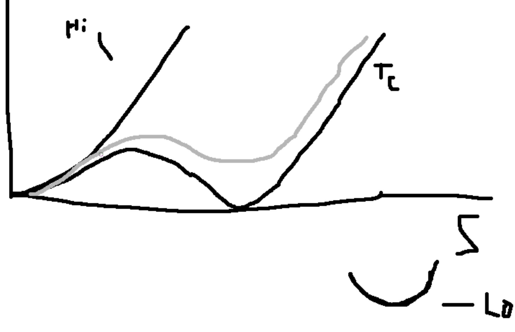
Consider the model, \(f = \frac{1}{2}r\phi^2 + u_4\phi^4 + u_6\phi^6\), \(u_6>0\) and \(u_4\) can be either sign. Plotting \(r\) versus \(u_4\),