Ising Model
Sites on a lattice with \(s_i\in\{\pm 1\}\) indexed by lattice site.
Then, \(E = -\sum_{j
C.f. Quantum mechanics \(J\hat{s}_i\cdot\hat{s}_j = \frac{J}{2}(S_{ij}^2-S_{i}^2-S_{j}^2)\) can be projected to a classical heisenberg model \(J\vec{s}_i\cdot\vec{s}_j\) and then project to 1D.
In our thermodynamic models, we can transition between a gas and a liquid without a phase transition… how? The ising model elucidates how.
Often consider nearest neighbor interaction only: \(E = -J\sum_{\langle ij\rangle}s_i\cdot s_j-B\sum_i s_i\).
This model cannot be used in dynamics, hence we don’t put a Hamiltonian, just E.
Qualitatively, what happens?
Suppose \(B=0\). If \(J>0\) and for low temperature then spins tend to be aligned with their nearest neighbors: \(\langle s_i\rangle\to \pm 1\). If \(J>0\) and we have high temperature then all of the states are roughly equally likely so they tend to be randomly oriented/ antialigned since there are more states: \(\langle s_i\rangle\to 0\).
Suppose \(J=0\). Then the spins align with the magnetic field hence if \(B=\pm 1\) then \(\langle s_i\rangle \to \pm 1\).
Solve \(B>0\) and \(J=0\).
\(E = -B\sum_i s_i = -BM\).
So, \(\langle E \rangle = N\langle \epsilon\rangle\). With \(\langle M\rangle = N\langle m\rangle\).
Choose \(N\) spins and a volume \(V\), note the volumetric dependence is in \(J\) since it relates to the neighbors.
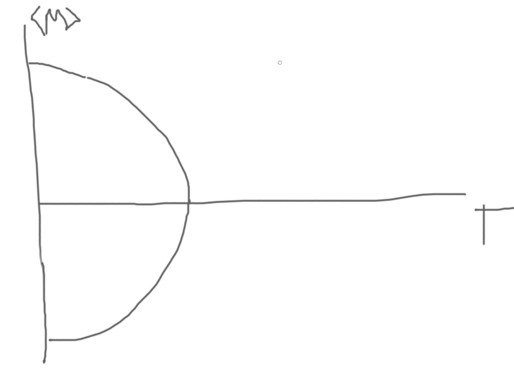
\(\langle m(T)\rangle = \langle s_i(T)\rangle = \frac{\langle M\rangle}{N}\) with \(M=\sum_i s_i\).
\(\langle s\rangle = \frac{\partial}{\partial (\beta B)}\)
\(\langle M\rangle = \frac{1}{Z}\sum_\alpha M_\alpha \exp(-E_\alpha/kT)\).
\(\langle m\rangle = \langle s\rangle = \frac{1}{Z}\sum _{i}s_i\exp(-\beta\epsilon_i) = \frac{\exp(-\beta(-B)) - \exp(\beta B)}{\exp(\beta B) + \exp(-\beta B)} = \frac{\exp(\beta B)-\exp(-\beta B)}{\exp(\beta B)+\exp(-\beta B)} = \text{tanh}(\beta B)\).
Let \(J>0\) and \(B=0\), \(E = -J\sum_{\langle i,j\rangle}s_is_j\).
\(E = -\frac{J}{2}\sum_i\sum_{k\in\{\text{nearest neighbor of site i}\}} s_is_k = -\frac{J}{2}\sum_i\left(s_i\sum_{n.n.}s_k\right) \approx -\frac{J}{2}\sum_i\left(s_i\left(\sum_{n.n.}\langle s\rangle\right)\right) = -\tilde{B}\sum_i s_i\) with \(\tilde{B} = Jz\langle s\rangle\) and \(z\) is the number of nearest neighbors. This is for looking at a single independent spin.
Then, \(m \approx \text{tanh}(\beta \tilde{B}) = \text{tanh}(\beta Jzm)\).
This is called a (naive) mean field approximation.
Note that the LHS is linear and the rhs is a tanh. Then \(m=0\) is always a solution. Further, we \(\tanh x \approx x-\frac{1}{3}x^3\). So, there could be a crossing at a finite \(T\) and \(m(T)\).
In this case, as \(T\) increases the slope decreases.
So at low temperature, we get a finite \(m\).
When the slopes meet, then we arrive at our final critical temperature.
\(T\to T_c\Rightarrow \frac{\partial LHS}{\partial m} = \frac{\partial RHS}{\partial m} \Rightarrow 1 \approx \frac{Jz}{kT_c}\) hence \(kT_c \approx Jz\).
Solving for \(m(T)\) near \(T_c\), \(m \approx \frac{Jz}{kT}m - \frac{1}{3}\left(\frac{Jz}{kT}m\right)^3\).
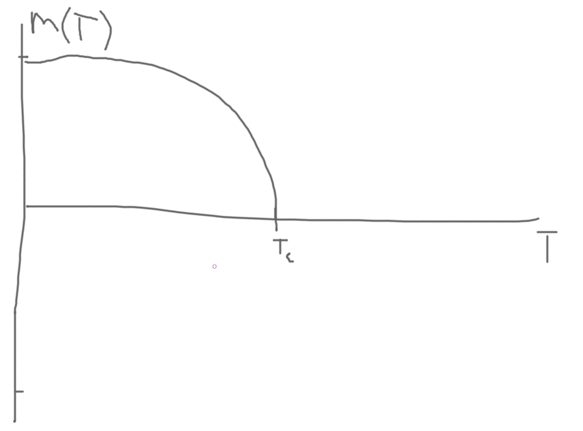
Then, \(\left(1-\frac{Jz}{kT}\right)\approx \frac{1}{3}\left(\frac{Jz}{kT}\right)^3m^2 \Rightarrow m(T) \approx \sqrt{\frac{3\left(1-\frac{Jz}{kT}\right)}{\left(\frac{Jz}{kT}\right)^3}} = \sqrt{3\left(1-\frac{T_c}{T}\right)\left(\frac{T}{T_c}\right)^3}\).
\(1-\frac{T_C}{T}=-\frac{1}{3}\left(\frac{T_C}{T}\right)^3m^2\).
Thus, \(m(T) = \pm\sqrt{3}\frac{T_C^{3/2}}{T^2}\sqrt{T_C-T}\)
Then, \(m\propto(T_C-T)^{\beta}\) with \(\beta = \frac{1}{2}\), \(T
The high temperature has more symmetry than the low temperature since rotating perspective around the lattice looks the same at high temperature rather than at low temperature where rotating can be distinguished.
High-temperature has the same symmetry as the Hamiltonian.
\(\beta-\) critical exponent.
\(C_B\propto |T-T_C|^{-\alpha}\), \(B=0\).
\(B,m=\frac{M}{N}\).
| \(\alpha\) |
\(C_B\) |
Heat Capacity, \(B=0,\alpha\to 0\) |
| \(\beta\) |
\(m\propto(T_C-T)^\beta\) |
Magnetization, \(T\to T_C, T
|
| \(\gamma\) |
\(\chi\propto \text{abs}(T-T_C)^\gamma\) |
\(B=0,\chi=\frac{1}{N}\left(\frac{\partial M}{\partial B}\right)_{B=0,T}\) |
| \(delta\) |
\(m\propto B^{1/\delta}\) |
\(B\to 0,T=T_C\). |
| \(\eta\) |
\(C_C^{(2)}(r)\propto\frac{1}{r^{d-2+\eta}}\) |
\(T=T_C,\beta=0\) |
| \(\nu\) |
\(\chi\propto\text{abs}(T-T_C)^{-\nu}\) |
\(T\) near \(T_C\), \(B=0\) and \(C_C^{(2)}\propto\exp(-r/\chi(T))\) |
\(C^{(2)}(\vec{r},t)\) is a correlation function \(\langle S(\overline{x},t)\cdot S(\overline{x}+\vec{r},t+\tau)\rangle\)
Equal time correlation, \(C^{(2)}(\vec{r},0)\). If we do this at infinite distance, \(C^{(2)}(\infty,0) = m^2\) since they are uncorrelated.
Then, \(C_C^{(2)}\) is the connected correlation function, which is \(C^{(2)} - C^{(2)}(\infty,0)\).
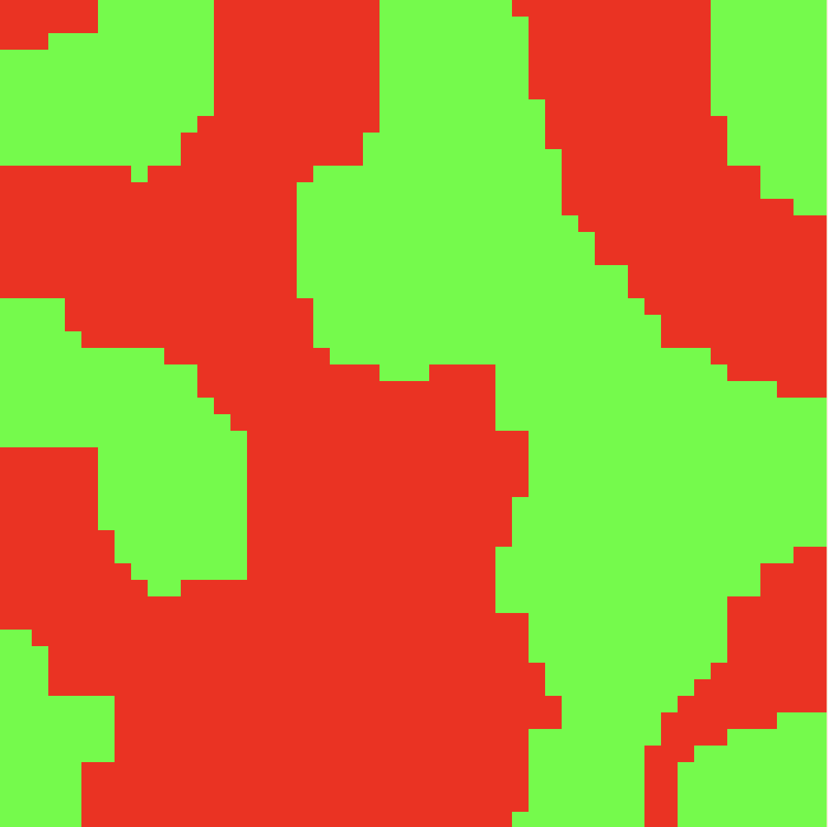 As you get lower temperature, regions of same spins start to appear.
1D \(z=2, kT_C = 2J, \beta=1/2\)
2D \(z=4, kT_C = 4J, \beta=1/2\)
3D \(z=6..12, kT_C \approx 8J, \beta=1/2\)
4D+ \(\beta=1/2\).
Exact solution:
1D. No transition
2D. \(kT_C = \frac{2J}{k_B\ln(1+\sqrt{2})} \approx 2.269J, \beta=1/8\).
3D. For Ferromagnets. Fe: \(\beta\approx 0.37\). Ni: \(\beta\approx 0.36\).
3D. \(\beta\approx 0.32(9)\).
4D+. \(\beta=1/2\).
Higher spin models are called Potts models.
Approximate Solutions for Low Temperature
Low Temperature is when we have the majority of occupations in the ground state, elementary exitation, or really close.
For a 1D ground state, all the spins being aligned, \(\epsilon_0\). Flipping one gives \(\Delta \epsilon = 4J\), hence \(\epsilon_1 = \epsilon_0+\Delta\epsilon\).
But wait, if we flip 2, then we get \(\epsilon_1 = \epsilon_0 + 2J\), hence the previous was the second exitation.
\(F(T,V,N) = E - TS\) with \(E = -J\sum_{i=0}^{N-1}s_is_{i+1}\).
\(F = -k\ln Z\) with \(Z = \sum_\alpha \exp(-\beta E_\alpha)\).
2 aligned states, \(2(N-1)\) with 1 neighbor pair flipped.
The average magnetization is zero.
\(\Delta F = F_1-F_0 = E_1 - E_0 - T(S_1 - S_0) = 2J - T(k\ln (N-1) - k\ln 1) = 2J - kT\ln (N-1)\).
For \(N\to \infty\), \(\Delta F < 0\).
For a 2D system.
Consider a domain wall with some boundary through the middle region.
For edge cases, the energy difference is \(2J\).
So, we get a minimum where \(\Delta E = 2J\cdot L\) where \(L\) is the length of the domain wall.
So, \(L\cong \tilde{c}_2N\) where \(\tilde{c}_2\approx 2\) to \(3\).
\(\tilde{c}_2\) denotes the number of choices of direction to go to the next lattice site.
Starting points is \(\tilde{c}_3N\).
Number of domain walls, \((\tilde{c}_2)^L\).
\(\tilde{c}_2=2,\tilde{c}_3=1\).
For \(\tilde{c}_2=2\) we get really close to exact result.
\(m = \langle s_0\rangle = f(\langle s_k\rangle)\) translational symmetry implies \(\langle s_0\rangle = \langle s_k\rangle\).
Then, \(m = \tanh(\beta (zJm+B))\).
A similar approach to calculating the Helmholtz free energy, \(F = U-TS\).
HW, Bragg-WIlliams approximation, see alloy section.
C.f. QM: Variational derivation of Mean Field Theory, MFT.
\(Z = \sum_\alpha\exp(-\beta H(\alpha))\) where \(\alpha\) denotes a configuration.
Split the Hamiltonian into two parts: \(H = H_0 + H_1\) such that we can evaluate \(Z_0\) for \(H_0\).
Then, we write, \(\frac{Z}{Z_0} = \frac{\sum_\alpha \exp(-\beta (H_0+H_1)_\alpha)}{\sum_\alpha\exp(-\beta H_0)} = \sum_{\alpha'}\frac{\exp(-\beta H_0(\alpha'))}{\sum_\alpha\exp(-\beta H_0(\alpha))}\exp(-\beta H_1(\alpha')) = \sum_{\alpha}p_0(\alpha)\exp(-\beta H_1(\alpha))\).
This gives the ensemble average with respect to the probability distribution \(p_0\), \(\frac{Z}{Z_0} = \langle\exp(-\beta H_1)\rangle_0\).
Now, \(\langle\exp(f)\rangle \geq\exp\langle f\rangle\).
Then, \(\frac{Z}{Z_0}\geq \exp\left(-\beta\langle H_1\rangle_0\right)\).
Hence, \(\ln Z - \ln Z_0 \geq -\beta\langle H_1\rangle_0\) with \(F=-kT\ln Z\) we get \(F\leq F_0 + \langle H_1\rangle_0\).
These two equations are the Bogolinbou or Gibs-Bog-Feynman inequalities.
Use \(F_0 = \langle H_0\rangle_0-TS_0\) with \(S_0 = -k\sum_\alpha p_\alpha\ln p_0\).
Then, \(F \leq \langle H_0\rangle_0 + \langle H_1\rangle_0 - TS_0\). Hence, \(F \leq \langle H\rangle_0 - TS_0\).
So, if you don’t have a total probability distribution, or not have one for one part, then you can compute an upper bound with what you do have.
Use independent particles (spin).
\(H_0 = \lambda\tilde{H}_0\) where \(\lambda\) is a variational parameter.
Then, \(F_{var}(\{\lambda_i\}) \equiv F_0(\lambda) + \langle H_1(\lambda)\rangle_0\).
Then, for our Ising model, \(H_0 = -\lambda\sum_i s_i\), we could have written \(\lambda B\), but for simplicity’s sake we absorb it.
Then, \(Z_0(\lambda) = [2\cos(\beta\lambda)]^N\) since for 1 spin, \(Z_1 = 2\cos\beta \tilde{B}\) and \(\langle s_1\rangle = \frac{2\sinh(\beta\tilde{B})}{2\cosh\beta\tilde{B}}= \tanh(\beta \tilde{B})\).
Then, \(H_1 = -J\sum_{\langle ij\rangle} + (\lambda-B)\sum_i s_i\).
Hence, \(\langle H_1\rangle_0 = -\frac{1}{2}zJN\langle s\rangle_0^2 + N(\lambda-B)\tanh(\beta\lambda) = -\frac{1}{2}NzJ\tanh^2(\beta\lambda) + N(\lambda-B)\tanh(\beta\lambda)\)
Note, \(F_1(\lambda) = -kT\ln Z_1(\lambda)\) so \(F_0 = NF_1\).
So, \(F_{var}(\lambda) = N\left(-\frac{1}{\beta}\ln(2\cosh\beta\lambda)\right)-\frac{1}{2}J\tanh^2(\beta\lambda)+(\lambda-B)\tanh(\beta\lambda)\).
Minimizing this, \(\frac{\partial F_{var}}{\partial \lambda}=0\) gives \(\lambda_{min} - B = zJ\tanh(\beta\lambda_{min})\).
Inserting this into the original expression, \(F_{var}(\lambda_{min}) = -\frac{N}{\beta}\ln(3\cosh(\beta\lambda_{min})) + \frac{N(\lambda_{min}-B)^2}{2zJ}\).
Then, \(m = -\frac{1}{N}\frac{\partial F}{\partial B} = -\frac{1}{N}\left(\frac{\partial F}{\partial B} + \frac{\partial F}{\partial\lambda}\frac{\partial\lambda}{\partial B}\right) = \frac{\lambda_{min}-B}{zJ} = \tanh(zJm+B)\).
Improve MF approach, general idea: cluster approximation(s).
Given a system, get a small ’core’ with a good ’exact’ solution. Solve surroundings in average way.
Can do this with dimensions, DMFT-Dynamical Mean Field Theory.
Example: Bethe Approximation.
1 spin. In MFT we have everything else as an averge. If we have a lattice we can model it with \(z=4\) neighbors.
The neighbor-of-neighbor(s) are mean field, averages.
So, consider the 1 spin \(s_0\) and the neighbor as \(s_k\), which is a sort of intermediate term.
\(E = -J\sum_{}s_is_j - B\sum_i s_i\).
Then the cluster energy is, \(E_c = -J\sum_{k=1}^z s_0s_k - Bs_0 - \tilde{B}\sum_{k=1}^zs_k\).
Compare MF, \(E_1 = -\tilde{B}s_0\), \(\tilde{B} = -Jzm\).
Now we calculate, \(\langle s_0\rangle\) and \(\langle s_k\rangle\), ’they are all the same’.
All spins are equal (translational symmetry), whyich gives \(\langle s_0\rangle = \langle s_k\rangle\) (HW).
Continuing this, you can also get \(\frac{\cosh^{z-1}(\beta(K+\tilde{B}))}{\cosh^{z-1}(\beta(J_1-\tilde{B}))} = \exp(2\beta\tilde{B})\).
Then, \(\frac{\partial LHS}{\partial\tilde{B}}_{\tilde{B}=0} = \frac{\partial RHS}{\partial\tilde{B}}_{\tilde{B}=0}\) so \(B_0J=\frac{1}{2}\ln\frac{Z}{Z-2}\). For a 2d lattice, \(kT_c=2.885J\) where the exact is \(2.269J\).
\(m(T)\propto (T_c-T)^\beta,\beta=1/2\) is always obtained but we get better \(kT_c\).
Setup for Next Time
Exact solutions:
- Open chain: \(E = -J\sum_{i=1}^{N01}s_is_{i+1}\). \(Z_N = \sum_{s_1=\pm1}\sum_{s_2=\pm1}\cdots\sum_{s_N=\pm1}\exp(-\beta(-J\sum_{i=1}^{N-1}s_is_{i+1}))\). So we get lots of products.
Since we have an open chain, you can start at the first or last chain, \(\exp(\beta J s_i s_{i+1})\exp(\beta J s_{i+1} s_{i+2})\sum_{s_N}\exp(\beta J s_{N-1} s_{N})\).
So, \(\exp(\beta Js_{N-1}) + \exp(-\beta Js_{N-1}) = 2\cosh(\beta J)\).
Now we have a new last spin, we can keep doing this and sum them up.
(HW) \(Z_n = 2(2\cosh(\beta J))^{N-1}, F = -kT\ln Z_n, U = -\frac{\partial\ln Z}{\partial\beta}, C_V = \frac{\partial U}{\partial T}\).
To avoid loops, \(1<\tilde{c}<3\) with \(c\approx 2\).
\(L = N\tilde{c} = Nc\) with \(N_{DW} = Nc^L\).
\(\Delta F = 2JL-kT\ln(Nc^L) = 2JcN-kT\ln(Nc^{NC}) = 2JNc - kT\ln N - NkTc\ln c = 2JNc-Nktc\ln c\).
For Ferromagnetic state, \(\Delta F = 2NJc - Nktc\ln c > 0\).
\(kTc = \frac{2J}{\ln c} > 0, \ln c > 0, c > 1\).
\(kTc \sim \{2.9J,c=2; 1.8J, c=3\}\)
Transfer Matrix Solution of One-Dimension Ising Model
Consider the transfer matrix solution to 1D ising model. For a ring arrangement.
\(E = -J\sum_{i=1}^Ns_is_{i+1}-B\sum_{i=1}^n s_i\).
Symmetrizing this \(i\Leftrightarrow i+1\), \(E = -\sum_{i=1}^N \left(Js_is_{i+1} + \frac{B}{2}(s_i+s_{i+1})\right)\).
So, \(Z_N = \sum_\alpha \exp(-\beta E),\alpha=\{s_1=\pm1,s_2=\pm1,\cdots,s_N=\pm1\}\).
Then, \(Z_N = \sum_{s_i}\prod_{i=1}^N\exp(\beta(Js_{i}s_{i+1}+\frac{B}{2}(s_i+s_{i+1})))\).
Hence, \(Z_N = \text{Tr}(T^N)\) solves our system.
We get the solution from diagonalizing the matrix, \(D = UTU^{-1}\) hence \(Z_N = \text{Tr}(T^N) = \text{Tr}(D^N)\).
Then, \(Z_N = \text{Tr}(T^N) = \lambda_1^N + \lambda_2^N + \cdots\) and \(F_N = -kT\ln Z_N = -kT\ln(\lambda_1^N + \lambda_2^N+\cdots)\).
Let \(\lambda_1\) be the largest.
Suppose we only have a 2x2,
\(F_N = NkT\ln\lambda_1 - kT\ln\left(1+\frac{\lambda_2^N}{\lambda_1^N}\right) \to NkT\ln\lambda_1\) in the thermodynamic limit.
Hence we only need the largest eigenvalue.
For \(N=2\),
\(Z_2 = \exp(\beta(J(-1)(-1)+\frac{B}{2}((-1)+(-1))))\exp(\beta(J(-1)(-1)+\frac{B}{2}((-1)+(-1)))) + \exp(\beta(J(-1)(1)+\frac{B}{2}((-1)+(1))))\exp(\beta(J(1)(-1)+\frac{B}{2}((1)+(-1)))) + \exp(\beta(J(1)(-1)+\frac{B}{2}((1)+(-1))))\exp(\beta(J(-1)(1)+\frac{B}{2}((-1)+(1)))) + \exp(\beta(J(1)(1)+\frac{B}{2}((1)+(1))))\exp(\beta(J(1)(1)+\frac{B}{2}((1)+(1))))\)
\(Z_2 = \exp(2\beta(J-B)) + \exp(2\beta J) + \exp(2\beta J) + \exp(2\beta(J+B))\)
We get \(2^N\) terms in sum of products of \(N=2\) exponentials.
From the board: \(\exp(++)\exp(++) + \exp(+-)\exp(-+) + \exp(-+)\exp(+-) + \exp(--)\exp(--)\)
So, \(Z_2 = \exp(2\beta(J+B)) + 2\exp(-2\beta J) + \exp(2\beta(J-B))\).
So, \(\text{Tr}(T^2) = \begin{pmatrix}
t_{11} & t_{12} \\
t_{21} & t_{22}
\end{pmatrix}\begin{pmatrix}
t_{11} & t_{12} \\
t_{21} & t_{22}
\end{pmatrix} = t_{11}^2 + 2t_{12}t_{21} + t_{22}^2\)
Then, \(T = \begin{pmatrix}
\exp(\beta(J+B)) & \exp(-\beta J) \\
\exp(-\beta J) & \exp(\beta(J-B))
\end{pmatrix}\).
The eigenvalues are then \(\lambda_{1/2} = \exp(\beta J)\cos(\beta B)\pm\sqrt{\exp(2\beta J\sinh(\beta B)+\exp(-2\beta J))}\).
\(F = -NkT\ln\lambda_1\), \(m = -\frac{1}{N}\frac{\partial F}{\partial B} = \frac{kT}{\lambda_1}\frac{\partial\lambda_1}{\partial B} = \frac{\sinh(\beta B)}{\sqrt{\sinh^2(\beta B)+\exp(-4\beta J)}}\).
For \(B=0\) then \(m=0\).
But even for a slight field, we get a non-zero field. I.e. for any \(B\neq 0\) we get \(\sinh^2(\beta B)\gg\exp(-4\beta J)\) hence \(m\to \pm 1\).
Calculate ensemble averages with a computer.
Monte Carlo
Ising model with \(N_S\) sites.
Then the number of configurations are \(N_\alpha = 2^{N_S}\).
For a 10x10 lattice, we get \(N_\alpha = 2^{100}\) which is more than the number of atoms in the observable universe.
If we choose states randomly, we tend to not get our ensemble average since most states are roughly zero magnetization.
As we get more samples, we get a narrower peak around zero and it will start to converge to zero magnetization.
With the heatbath method we no longer need to calculate the probability (boltzman factor and normalization) distribution for random samples.
Heat Bath MC
Pick a spin in the lattice \(s_i = (n_x,n_y)\).
Count number of up spins among neighbors: \(n_i\).
Compute \(m_i = \sum_{j\in n_i}s_j\).
| \(m_i\) |
\(n_i\) |
| 4 |
4 |
| 2 |
3 |
| 0 |
2 |
| -2 |
1 |
| -4 |
0 |
Compute energy of spin \(i\) given the environment.
\(E_{+} = -Jm_i - B\)
\(E_{-} = Jm_i + B\)
Set spin \(s_i = +1\) with \(p_+ = \frac{\exp(-\beta E_+)}{\exp(-\beta E_+) + \exp(-\beta E_-)}\) or \(s_i=-1\) with \(p_- = \frac{\exp(-\beta E_-)}{\exp(-\beta E_+) + \exp(-\beta E_1)}\).
Record \(E_n;M_N\).
Repeat \(N\) times.
\(\langle E\rangle = \frac{1}{N}\sum_{n=1}^N E_n, \langle M\rangle = \frac{1}{N}\sum_{n=1}^N M_n\).
Keep track of \(E_n^2\) and \(M_n^2\) for variances and response function.
Monte Carlo
Sampling: Estimate of \(\langle x\rangle\).
Randomly generating \(B\) configurations of the system. Let \(E[x]\) be the estimator of \(\langle x\rangle\).
Then, \(E[x] = x_B = \frac{\frac{1}{B}\sum_i^B x_{\alpha i}\exp(-\beta E_{\alpha i})}{\frac{1}{B}\sum_i^B\exp(-\beta E_{\alpha i})}\).
Unbiased: \(p_\alpha = \frac{1}{N_\alpha}\). Then, \(\frac{1}{B}\sum_{i=1}^B\sum_{n=1}^{N_\alpha}\frac{1}{N_\alpha}\exp(-\beta E_{\alpha n}) = \frac{B}{B}\frac{1}{N_\alpha}Z\) and \(\frac{1}{B}\sum_{i=1}^B\sum_{n=1}^{N_\alpha}\frac{x_\alpha}{N_\alpha}\exp(-\beta E_{\alpha n}) = \frac{B}{B}\frac{1}{N_\alpha}Z\langle x\rangle\).
For an unbiased estimator, \(\langle E[x]\rangle = \langle x\rangle\)
Choose configuration \(\alpha_n\) with probability \(\propto \exp\left(-\beta E_{\alpha n}\right)\), \(E[x] = \frac{1}{B}\sum_{i=1}^B x_{\alpha i},\langle E[x]\rangle = \langle x\rangle\).
Example of importance sampling.
Markov Chain
Definition: Sequence of configurations generated by a Markov step.
Definition of a Markov step: Generates configuration based on the previous step only, not any prior. No memory effects.
We can describe a Markov step by \(N_\alpha^2\) probabilities from \(P(\beta\leftarrow\alpha) = P_{\beta\alpha}\).
Conditions for a Markov chain with a desired probability distribution \(p_\alpha\):
- \(\sum_\beta P(\beta\leftarrow\alpha)=1\), i.e. the system must go somewhere.
- Accesibility Condition: for a given configuration you must be able to get any other configuration in a finite number of steps
- Detailed Balance: \(p_\alpha P(\beta\leftarrow\alpha) = p_\beta P(\alpha\leftarrow\beta)\).
So, \(\frac{P(\beta\leftarrow\alpha)}{P(\alpha\leftarrow\beta)} = \frac{p_\beta}{p_\alpha}\).
For a Boltzman distribution (MB statistics), \(=\exp\left(-\frac{E_\beta-E_\alpha}{kT}\right)\).
Let \(\rho_\alpha(n)\) be the probability of the n-th element in the Markov chain to be configuration \(\alpha\).
Need to show \(\rho_\alpha(n)\) converges to \(p_\alpha\) for increasing \(n\) and that if we are at convergence that \(\rho_\alpha(n + \delta n)\) remains equal to \(p_\alpha\).
Formulation in terms of vectors and matrices.
\(\overline{\rho}_\alpha(n) = \begin{pmatrix}
p_1(n) \\
p_2(n) \\
\cdots \\
p_{N_\alpha}(n)
\end{pmatrix},P_{\beta\alpha}=\begin{pmatrix}
P(1\leftarrow 1) & P(1\leftarrow 2) & \cdots \\
P(2\leftarrow 1) & \cdots & \cdots \\
\cdots & \cdots & \cdots
\end{pmatrix}\).
Proving the second one first, suppose \(\rho_\alpha(n) = p_\alpha\). Then \(\rho_\alpha(n+1) = \sum_{\alpha '} p_{\alpha'}P(\alpha\leftarrow\alpha') = \sum_{\alpha'}p_\alpha P(\alpha'\leftarrow\alpha) = 1\).
Proving the first one.
Suppose \(\rho_{\alpha}(n) \neq p_\alpha\).
Let \(D_n\equiv \sum_\alpha |\rho_\alpha(n)-p_\alpha|\) be the norm we will work with.
Compute \(D_{n+1}\).
We want \(D_{n+1}\leq D_{n}\).
So,
\begin{align*}
D_{n+1}
&= \sum_\alpha|\rho_\alpha(n+1)-p_\alpha| \\
&= \sum_\alpha |\sum_{\alpha'} \rho_{\alpha'}(n)P(\alpha\leftarrow\alpha')-p_\alpha| \\
&= \sum_\alpha |\sum_{\alpha'} \rho_{\alpha'}(n)P(\alpha\leftarrow\alpha')-\sum_{\alpha'}P(\alpha\leftarrow\alpha)p_\alpha| \\
&= \sum_\alpha |\sum_{\alpha'} \rho_{\alpha'}(n)P(\alpha\leftarrow\alpha')-P(\alpha\leftarrow\alpha)p_\alpha| \\
&= \sum_\alpha|\sum_{\alpha'}(\rho_{\alpha'}(n)-p_\alpha)P(\alpha\leftarrow\alpha')| \\
&\leq \sum_\alpha\sum_{\alpha'}|(\rho_{\alpha'}(n)-p_\alpha)P(\alpha\leftarrow\alpha')| \\
&= \sum_\alpha\sum_{\alpha'}|(\rho_{\alpha'}(n)-p_\alpha)|P(\alpha\leftarrow\alpha') \\
&= \sum_{\alpha'}|(\rho_{\alpha'}(n)-p_\alpha)|\sum_\alpha P(\alpha\leftarrow\alpha') \\
&= \sum_{\alpha'}|(\rho_{\alpha'}(n)-p_\alpha)| \\
&= D_n
\end{align*}
Metropolis Monte Carlo
Situation: identical to heat-bath MC.
We can get the transition probability from probability distribution of initial and final states.
- Pick random spin
- Count how many neighbors are the same as the picked spin
Make a list
| \(\Delta n\) |
\(\Delta E\) |
Number of spins after |
Number of spins before |
| -4 |
8J |
0 |
4 |
| -2 |
4J |
1 |
3 |
| 0 |
0 |
2 |
2 |
| 2 |
-4J |
3 |
1 |
| 4 |
-8J |
4 |
0 |
Metropolis Choice: \(\Delta E\leq 0\) then we will flip the spin, otherwise flip with probability \(\exp(-\beta\Delta E)\).
Showing detailed balance:
Case 1. \(E_{-}
Note: If you want to simulate a high-temperature system then it is best to use another algorithm (see Galuber) since this will lead to always flipping a random spin.
\(\rho_\beta(n+1) = \sum_\alpha P(\beta\leftarrow\alpha)\rho_\alpha(n) = \sum_\alpha P_{\beta\alpha}\rho_\alpha(n)\).
So, \(\vec{\rho}(n+1) = P\vec{\rho}(n)\) hence at steady state \(\vec{\rho}^* = P\vec{\rho}^*\) with \(P\) now being a matrix and \(\vec{\rho}^*\) being an eigenvector of 1.
Theorem (1+2): At least one eigenvalue, \(\lambda^*\), is 1 all other eigenvaluses have eigenvectors orthogonal to it. So, \(\sum_{\lambda\neq\lambda^*}\lambda = 0\).
Theorem (3): \(\lambda = 1\) and all other \(|\lambda|<1\).
Theorem (4): Ergodic systems have only one \(\lambda = 1\).
\(\vec{\rho}(n) = P\vec{\rho}(n-1) = P^n\vec{\rho}(0)\). Expanding around \(\rho^*\),
\(\vec{\rho}(n) = \alpha_*\vec{\rho}^* + \sum_{|\lambda|<1} \alpha_\lambda\vec{\rho}^\lambda = \alpha_*\vec{\rho}^* + \sum_{|\lambda|<1} \alpha_\lambda\lambda^{n}\vec{\rho}(0)\).
Markovian System that does not obey Detailed Balance
COMPUTATIONAL PROBLEM.
Assume we have 1000 indistinguishable bacteria, 500 green and 500 red.
Every hour:
- Every bacteria divides
- Colorblind predator eats exactly 1000 bacteria
1001 possible states (0-1000 of one color).
Stationary state: 1/2 0 of 1 color and 1/2 1000 of 1 color, \(p^{st} = \frac{1}{2}R_0 + \frac{1}{2}R_{1000}\).